
A Practical Guide to Dynamic Programming (DP)
Ever wanted an algorithm to write an algorithm? Well, I did :) So I wrote this practical guide to DP (based on my personal experience)!
Introduction
DP is a really fascinating programming technique. It solves even the seemingly daunting problems in a linear time! Usually, problems that require you to calculate the amount of ways to solve a problem or to find the best way to solve a problem can be worked out with DP.
But, how does it work?
Well, actually, DP is an application of brute-forcing because it tries every single possible ways to solve a problem. However, this brute-force is optimized by storing the result of already solved sub-problems that the program previously encountered.
DP can be used in place of the greedy technique. The difference between the two, is that with DP, you’d have to map out every possible ways to solve a problem (and either pick the optimum one or count the ways), while with greedy, the optimum way to solve the problem is already known. An algorithm utilizing DP is easier to factual-check because it would’ve seen every of the possible ways to solve a problem, so it is guaranteed that you get the most optimum result.
There are two ways to implement dynamic programming:
-
Top-down
A top-down implementation of DP is done recursively by solving the biggest problem first where we don’t know the solution to our problem yet. We then recursively go solve each one of those, ensuring that we only try to calculate the function call with a particular parameter once. This is done using memoization.
-
Bottom-up
A bottom-up implementation of DP is done by solving the problem that we already know the solution of. Then, we work our way up until we go to our main/biggest problem. This is done by tabulating the result.
Approaching a DP Problem
Here are my steps to solve a problem with DP:
- Think about how you would build the solution systematically by hand. Since DP is just a brute-forcing algorithm, do not worry about how unoptimized it is—it will be anyways :)
- Write down the recursive formula for the problem, making use of what’s already known from the solved sub-problems.
- Determine its base case, i.e a specific sub-problem whose solution is already known.
- Implement its solution or calculate it.
Example Case: Building a Number String
Let’s go through an example problem.
Given an array {0, 1, 2}, How many ways are there to create N-length string using the three possible numbers for each character, where each character is only allowed to have at most 1 difference from its neighboring character?
Example (N = 2):
{0, 0}, {0, 1}, {1, 0}, {1, 1}, {1, 2}, {2, 1}, {2, 2} = 7 ways
Building By-Hand
How would one manually build a string of length N with the said rules?
We’d want to loop from the first character to the last one. For N = 1 (i.e same thing—the first character), we only have three ways: {0}, {1}, and {2}.
Now, notice that we’re going to have to take the next step(s) differently depending on which number we pick. If we had picked 0, we only have choices {0} and {1} for the next character. If we had picked {1}, we’d have {0}, {1}, and {2}. If we had picked {2}, we’d have {1} and {2}.
So now, when we try to map out the amount of possibilities that we’re gonna have, we get this:
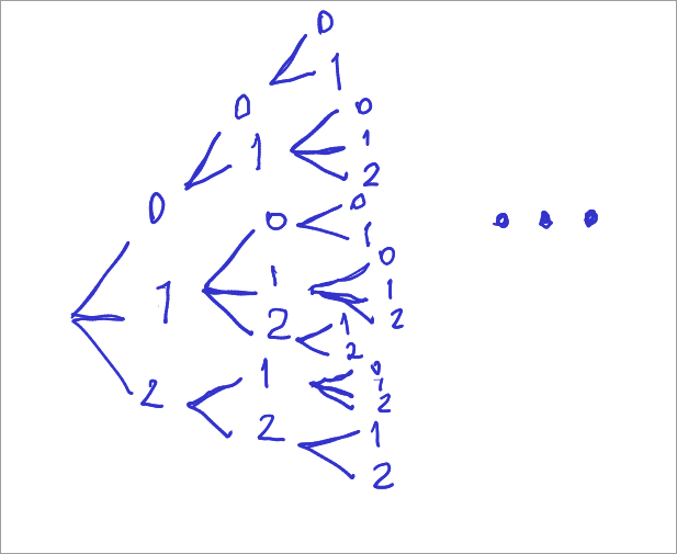
And to get the amount of proper arrangements, we’d just have to calculate all the amount of nodes in that tree.
Recursive Formula
To get our formula, we’d first have to ask, what is our sub-problem exactly?
The main rule of the formula-crafting is that it must not discriminate between differences of parameter, i.e all those 0, 1, and 2’s must be of the same sub-problem.
A helpful way to get our sub-problem is to go to our last step. Assume we’re at the edge of our problem-solving, i.e we’re at the last character. What exactly are we going to do? We are writing the (last) possible character from the choices that we have. And that, is our sub-problem, because (see below) it is recursive (i.e you need to answer a similar sub-problem to get that answer).
Our new question would be: how many ways are there to write the last possible character from the choices that we have? Intuitively, it’s just the ways to append 0 + the ways to append 1 + the ways to append 2.
But, comes the next problems. We don’t even know how to calculate those. So let’s jump through all of them:
-
To append 0
We aren’t always able to write 0. We can only write 0 if our previous character was 0 or 1. Therefore, the total ways to write 0 when length is $ x $ is the ways to write 0 with length $ x-1 $ + the ways to write 1 with length $ x-1 $. Those are all the possibilities that make us able to write 0 at position $ x $.
-
To append 1
Same thing here, we can only write 1 if our previous character was 0, 1, or 2. The ways to write 1 when length is $ x $ is the ways to write 0 with length $ x-1 $ + the ways to write 1 with length $ x-1 $ + the ways to write 2 with length $ x-1 $.
-
To append 2
Also the same. The ways to write 2 when length is $ x $ is the ways to write 1 with length $ x-1 $ + the ways to write 2 with length $ x-1 $.
Let’s simplify a bit. Assume that the solution to our original question is defined as f(x). And:
- a(x): ways to append 0 with length x
- b(x): ways to append 1 with length x
- c(x): ways to append 2 with length x
Therefore:
- f(x) = a(x) + b(x) + c(x)
- a(x) = a(x-1) + b(x-1)
- b(x) = a(x-1) + b(x-1) + c(x-1)
- c(x) = b(x-1) + c(x-1)
Making Our Base Case(s)
We have to make our recursion finite, so we need a base case. A base case is a problem whose solution is already known.
Now, it’s helpful to go to the start of the problem instead in this case–when we don’t have anything yet. When we first append a character (this is f(x)), there’s only 3 choices: append 0, 1, or 2. Or, in other words, f(1) = 3.
But since f(x) is composed out of a(x), b(x), and c(x), it’s a lot more helpful to find the base cases for those functions:
-
a(x)
When x = 1, it means the amount of ways to append 0 with length 1. There’s nothing previously, so obviously, there’s only one way to append 0 which is our first step in building our string.
-
b(x)
Same thing as above. There’s only one way.
-
c(x)
Same thing as above.
Now this does check out, as f(x) = a(x) + b(x) + c(x) and f(1) = 1 + 1 + 1 = 3.
Our Formula
\[f(x) = \begin{cases} a(x) + b(x) + c(x) & \text{if x > 1} \\ 3 & \text{if x = 1} \end{cases}\]And
\[a(x) = \begin{cases} a(x-1) + b(x-1) & \text{if x > 1}\\ 1 & \text{if x = 1} \end{cases}\] \[b(x) = \begin{cases} a(x-1) + b(x-1) + c(x-1) & \text{x > 1}\\ 1 & \text{if x = 1} \end{cases}\] \[c(x) = \begin{cases} b(x-1) + c(x-1) & \text{if x > 1}\\ 1 & \text{if x = 1} \end{cases}\]Calculating & Implementation
I’ll use bottom-up DP to fill a table, then display all the function call values (C++). Bottom-up approach is usually more preferred as we don’t get affected by function call overhead—and we can do a lot more interesting stuff with it!
Disclaimer: why C++? It’s nice for competitive programming scripts haha
#include <iostream>
using namespace std;

int main() {
	int N;
	cin >> N;
	int f[N+1];
	int a[N+1];
	int b[N+1];
	int c[N+1];

	a[1] = 1;
	b[1] = 1;
	c[1] = 1;

	f[1] = a[1] + b[1] + c[1];

	cout << "f(" << 1 << ") = " << f[1] << "\n";

	for (int i = 2; i <= N; i++) {
		a[i] = a[i-1] + b[i-1];
		b[i] = a[i-1] + b[i-1] + c[i-1];
		c[i] = b[i-1] + c[i-1];
		f[i] = a[i] + b[i] + c[i];
		cout << "f(" << i << ") = " << f[i] << "\n";
	}
}
So now, when we give some value for N:
$> ./program
10
f(1) = 3
f(2) = 7
f(3) = 17
f(4) = 41
f(5) = 99
f(6) = 239
f(7) = 577
f(8) = 1393
f(9) = 3363
f(10) = 8119
it will print the filled table.
Complexity Analysis
The time complexity of this is always O(N), as the loop iterates over N times. The space complexity, however, is O(N) as well because we store all the resulting solution of our sub-problems. We will optimize it in the next section.
Optimizing
Notice that we only need to access our previous result, because in all our recurrence relations, we only use the parameter $ x-1 $.
This means that storing the whole table is redundant, as we can simply only store the previous result:
#include <iostream>
using namespace std;

int main() {
	int N;
	cin >> N;
	int a_prev = 1;
	int b_prev = 1;
	int c_prev = 1;
	int f_prev = a_prev + b_prev + c_prev;

	int f, a, b, c;

	cout << "f(" << 1 << ") = " << f_prev << "\n";

	for (int i = 2; i <= N; i++) {
		a = a_prev + b_prev;
		b = a_prev + b_prev + c_prev;
		c = b_prev + c_prev;
		f = a + b + c;
		cout << "f(" << i << ") = " << f << "\n";

		a_prev = a;
		b_prev = b;
		c_prev = c;
		f_prev = f;
	}
}
And with this, we get O(N) time complexity and O(1) space complexity. Awesome!